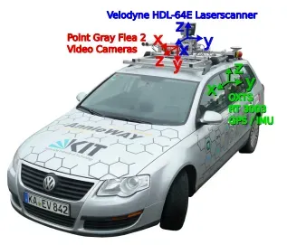
A perpetual pain point for people working on computer vision is dealing with affine transformations. Usually you have a diagram that looks something like this:

Each of the coordinate frames can be represented as a 4x4 matrix in Numpy. For the three sensors in the image above we might have something like this:

T_world_to_lidar # 4x4
T_world_to_camera # 4x4
T_world_to_imu # 4x4

Suppose we have a point p in the world frame. We can transform it to one of the other frames using matrix multiplication:

p = np.array([x, y, z, 1])
p_lidar = T_world_to_lidar @ p  # 4x4 @ 4x1 = 4x1

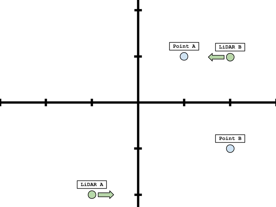
Here’s a toy example in 2D to illustrate the concept:

p_a_in_world = np.array([1, 1])
p_b_in_world = np.array([2, -1])

T_world_to_lidar_a = np.array([
    [1, 0, 1],
    [0, 1, 2],
    [0, 0, 1],
])

T_world_to_lidar_b = np.array([
    [-1, 0, 2],
    [0, -1, 1],
    [0, 0, 1],
])

p_a_in_lidar_a = T_world_to_lidar_a @ np.append(p_a_in_world, 1)   # [2, 3]
p_b_in_lidar_a = T_world_to_lidar_a @ np.append(p_b_in_world, 1)   # [3, 1]
p_a_in_lidar_b = T_world_to_lidar_b @ np.append(p_a_in_world, 1)   # [1, 0]
p_b_in_lidar_b = T_world_to_lidar_b @ np.append(p_b_in_world, 1)   # [0, 2]

p_o_in_lidar = np.array([0, 0])
p_o_a_in_world = np.linalg.inv(T_world_to_lidar_a) @ np.append(p_o_in_lidar, 1)  # [-1, -2]
p_o_b_in_world = np.linalg.inv(T_world_to_lidar_b) @ np.append(p_o_in_lidar, 1)  # [2, 1]

In words:

• point_a in the world frame is (1, 1) and point_b in the world frame is (2, -1)
• After multiplying the point by the transformation matrix, we get where the points are from each LiDAR’s perspective:
  • point_a in LiDAR A’s frame is (2, 3)
  • point_b in LiDAR A’s frame is (3, 1)
  • point_a in LiDAR B’s frame is (1, 0)
  • point_b in LiDAR B’s frame is (0, 2)
• We can get each LiDAR’s position in the world frame by applying the inverse transformation to the origin:
  • LiDAR A is at (-1, -2)
  • LiDAR B is at (2, 1)

Here’s how this looks visually, where the axis has the origin at the world frame: