Diffusion verses Flow Matching

This post is a summary of a couple of generative modeling papers recently that have been impactful. I’m primarily writing this for my own understanding, but hopefully it’s useful to others as well, since this is a fast-paced area of research and it can be hard to dive deeply into each new paper that comes out.

This post uses what I’ll call “math for computer scientists”, meaning there will likely be a lot of abuse of notation and other hand-waving with the goal of conveying the underlying idea more clearly. If there is a mistake (and it looks unintentional) then let me know!

All Papers

This post will discuss three papers:

• Diffusion from Denoising Diffusion Probabilistic Models
• Latent Diffusion from High-Resolution Image Synthesis with Latent Diffusion Models (a.k.a. the Stable Diffusion paper)
• Flow Matching from Flow Matching for Generative Modeling

Other Good References

• What are diffusion models? from Lil’ Log
• Diffusion Models from Scratch from Tony Duan

Application Links

• Diffusion Distillation from Progressive Distillation for Fast Sampling of Distillation Models
• Simple Diffusion from simple diffusion: End-to-end diffusion for high resolution images
• Autoregressive Diffusion from Autoregressive Diffusion Models
• On the Importance of Noise Scheduling for Diffusion Models
• Voicebox from Voicebox: Text-Guided Multilingual Universal Speech Generation at Scale
• Collection of Speech Synthesis Papers

These papers overlap and cite each other in various ways.

Diffusion

Diffusion models can be summarized very shortly as:

1. Start with a random image.
2. Iteratively add noise to the image.
3. Train a model to predict some part of the noise that was added.
4. Iteratively remove noise from the image by predicting and subtracting it.

Consider Figure 2 from the original paper:

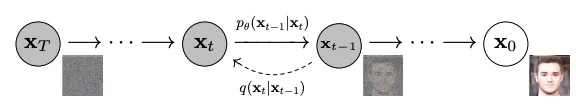
In the above diagram:

• $x_T$ is some noise, typically Gaussian noise
• $x_0$ is the original image
• $p_{\theta}(x_{t-1}|x_t)$ is called the reverse process, a distribution over the sligtly less noisy image given the current image
• $q(x_t|x_{t-1})$ is called the forward process, a Markov chain that adds Gaussian noise to the data

How do we convert a regular image to Gaussian noise?

Let’s assume we have a noisy image $x_{t-1}$ and we want to make it slightly noisier (in other words, take a step along the forward process, $q(x_t|x_{t-1})$). We sample the slightly noisier image $x_t$ from the following distribution:

$x_t \sim \mathcal{N}(\sqrt{1 - \beta_t} x_{t - 1}, \beta_t \textbf{I})$

This can be read as, “sample $x_t$ from a Gaussian distribution with mean $\sqrt{1 - \beta_t} x_{t - 1}$ and variance $\beta_t \textbf{I}$.” The matrix $\textbf{I}$ is just the identity matrix, so $\beta_t$ is the variance of the Gaussian noise being added.

Recall that the sum of two Gaussian distributions is also a Gaussian distribution:

$\begin{aligned} X & \sim \mathcal{N}(\mu_Y, \sigma_X^2) \\ Y & \sim \mathcal{N}(\mu_Y, \sigma_Y^2) \\ X + Y & \sim \mathcal{N}(\mu_X + \mu_Y, \sigma_X^2 + \sigma_Y^2) \end{aligned}$

It’s also worth noting that multiplying a zero-mean Gaussian by some factor $\alpha$ is equivalent to multiplying the variance by $\alpha^2$:

$\alpha \mathcal{N}(\textbf{0}, \textbf{I}) = \mathcal{N}(\textbf{0}, \alpha^2 \textbf{I})$

So we can rewrite the distribution from earlier as:

$\begin{aligned} \mathcal{N}(\sqrt{1 - \beta_t} x_{t - 1}, \beta_t \textbf{I}) & = \mathcal{N}(\sqrt{1 - \beta_t} x_{t - 1}, \textbf{0}) + \mathcal{N}(\textbf{0}, \beta_t \textbf{I}) \\ & = \sqrt{1 - \beta_t} x_{t - 1} + \sqrt{\beta_t} \mathcal{N}(\textbf{0}, \textbf{I}) \end{aligned}$

This is our forward process $q(x_t|x_{t-1})$:

$q(x_t|x_{t-1}) = \sqrt{1 - \beta_t} x_{t - 1} + \sqrt{\beta_t} \mathcal{N}(\textbf{0}, \textbf{I})$

So, to recap, in order to convert a regular image to Gaussian noise, we repeatedly apply the $q(x_t|x_{t-1})$ rule to add noise to the image, and $T \to \infty$ will result in a random distribution of noise.

The variances for each step of the $q$ update is given by some schedule $\beta_1, \beta_2, \dots, \beta_T$. The schedule is typically linearly increasing from 0 to 1, so that on the final step when $\beta_T = 1$ we will sample a completely noisy image from the distribution $\mathcal{N}(\textbf{0}, \textbf{I})$.

How do you sample $x_t$ in closed form (i.e., without sampling $x_{t - 1}, ..., x_{1}$)?

Rather than having to take our original image and run 1 to $T$ steps to get a noisy image, we can use the reparametrization trick.

If we start with our original image $x_0$, we can write the first slightly noisy image $x_1$ as:

$\begin{aligned} x_1 & = \sqrt{1 - \beta_1} x_0 + \mathcal{N}(\textbf{0}, \beta_1 \textbf{I}) \\ & = \sqrt{1 - \beta_1} x_0 + \sqrt{\beta_1} \mathcal{N}(\textbf{0}, \textbf{I}) \\ \end{aligned}$

We can rewrite this using $\alpha_t = 1 - \beta_t$ as:

$x_1 = \sqrt{\alpha_1} x_0 + \mathcal{N}(\textbf{0}, (1 - \alpha_1) \textbf{I})$

We can then write $x_2$ as:

$\begin{aligned} x_2 & = \sqrt{\alpha_2} x_1 + \mathcal{N}(\textbf{0}, (1 - \alpha_2) \textbf{I}) \\ & = \sqrt{\alpha_2} (\sqrt{\alpha_1} x_0 + \mathcal{N}(\textbf{0}, (1 - \alpha_1) \textbf{I})) + \mathcal{N}(\textbf{0}, (1 - \alpha_2) \textbf{I}) \\ & = \sqrt{\alpha_1 \alpha_2} x_0 + \mathcal{N}(\textbf{0}, \alpha_2 (1 - \alpha_1) \textbf{I}) + \mathcal{N}(\textbf{0}, (1 - \alpha_2) \textbf{I}) \\ & = \sqrt{\alpha_1 \alpha_2} x_0 + \mathcal{N}(\textbf{0}, (\alpha_2 (1 - \alpha_1) + (1 - \alpha_2)) \textbf{I}) \\ & = \sqrt{\alpha_1 \alpha_2} x_0 + \mathcal{N}(\textbf{0}, (1 - \alpha_1 \alpha_2) \textbf{I}) \\ \end{aligned}$

This can be extended recursively¹, so we can write $x_t$ in closed form as:

$x_t = \sqrt{\alpha_1 \alpha_2 \dots \alpha_t} x_0 + \mathcal{N}(\textbf{0}, (1 - \alpha_1 \alpha_2 \dots \alpha_t) \textbf{I})$

It’s common to express the product as a new variable:

$\bar{\alpha}_t = \alpha_1 \alpha_2 \dots \alpha_t = \prod_{i=1}^{t} \alpha_i$

Also, the usual notation is to write $\epsilon_t \sim \mathcal{N}(\textbf{0}, \textbf{I})$, giving the final equation for sampling $x_t$ as:

$x_t = \sqrt{\bar{\alpha}_t} x_0 + \sqrt{1 - \bar{\alpha}_t} \epsilon_t$

Sampling $\epsilon_t$ from $\mathcal{N}(\textbf{0}, \textbf{I})$ and using it to derive $x_t$ is called Monte Carlo sampling. Alternatively, we can use our $q$ notation from earlier to specify the closed-form distribution that the sample is drawn from:

$\begin{aligned} q(x_t | x_0) & = \sqrt{\bar{\alpha}_t} x_0 + \sqrt{1 - \bar{\alpha}_t} \mathcal{N}(\textbf{0}, \textbf{I}) \\ & = \mathcal{N}(\sqrt{\bar{\alpha}_t} x_0, (1 - \bar{\alpha}_t) \textbf{I}) \\ \end{aligned}$

How is the model trained?

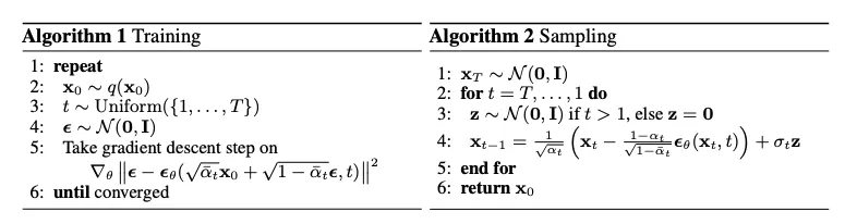
The main goal of the learning process is to maximize the likelihood of the data after repeatedly applying the reverse process. First, we sample some noise $\epsilon_t \sim \mathcal{N}(\textbf{0}, \textbf{I})$ and then we apply the forward process $q(x_t | x_0)$ to get $x_t$:

$x_t = \sqrt{\bar{\alpha}_t} x_0 + \sqrt{1 - \bar{\alpha}_t} \epsilon_t$

The diffusion model training process involves training a model which takes $x_t$ and $t$ as input and predicts $\epsilon_t$:

$\hat{\epsilon}_t = \epsilon_{\theta}(x_t, t)$

We can train the model to minimize the mean squared error between $\epsilon_t$ and $\hat{\epsilon}_t$:

$\mathcal{L} = ||\epsilon_t - \hat{\epsilon}_t||^2$

So, the model is predicting the noise between the noisy image and the original image.

How do you sample from the model?

Now that we’ve ironed out the math for the forward process, we need to flip it around to get the reverse process. In other words, given that we have $q(x_t | x_{t-1})$, we need to derive $q(x_{t-1} | x_t)$ ². The first step is to apply the chain rule:

$\begin{aligned} q(x_{t-1} | x_t) & = \frac{q(x_t | x_{t-1}) q(x_{t-1})}{q(x_t)} \\ & \propto q(x_t | x_{t-1}) q(x_{t-1}) \\ \end{aligned}$

We drop the denominator because $x_t$ is constant when we are sampling.

Recall the probability density function for a normal distribution:

$\mathcal{N}(x | \mu, \sigma^2) = \frac{1}{\sqrt{2 \pi \sigma^2}} \exp(-\frac{(x - \mu)^2}{2 \sigma^2})$

We can use this to rewrite $q(x_t | x_{t-1})$ as a function of $x_{t-1}$:

$\begin{aligned} q(x_t | x_{t-1}) & = \mathcal{N}(x_t | \sqrt{\bar{\alpha}_t} x_{t-1}, (1 - \bar{\alpha}_t) \textbf{I}) \\ & = \frac{1}{\sqrt{2 \pi (1 - \bar{\alpha}_t)}} \exp(-\frac{(x_t - \sqrt{\bar{\alpha}_t} x_{t-1})^2}{2 (1 - \bar{\alpha}_t)}) \\ \end{aligned}$

Similarly for $q(x_{t-1})$:

$\begin{aligned} q(x_{t-1}) & = \mathcal{N}(x_{t-1} | \sqrt{\bar{\alpha}_{t-1}} x_0, (1 - \bar{\alpha}_{t-1}) \textbf{I}) \\ & = \frac{1}{\sqrt{2 \pi (1 - \bar{\alpha}_{t-1})}} \exp(-\frac{(x_{t-1} - \sqrt{\bar{\alpha}_{t-1}} x_0)^2}{2 (1 - \bar{\alpha}_{t-1})}) \\ \end{aligned}$

Anyway, somehow if you do some crazy math you can eventually arrive at the equations for the forward process, which are:

$x_{t - 1} = \frac{1}{\sqrt{\alpha_t}}(x_t - \frac{1 - \alpha_t}{\sqrt{1 - \bar{\alpha}_t}} \epsilon_{\theta}(x_t, t)) + \sigma_t z$

where $z \sim \mathcal{N}(\textbf{0}, \textbf{I})$ is new noise to add at each step and $\epsilon_{\theta}(x_t, t)$ is the output of the model.

Latent Diffusion

The latent diffusion paper is most notable because it produces high-quality image samples with a relatively simple model. It contains two training phases:

1. Autoencoder to learn a lower-dimensional latent representation
2. Diffusion model learned in the latent space

The main insight is that learning a diffusion model in the full pixel space is computationally expensive and has a lot of redundancy. Instead, we can first obtain a lower-rank representation of the image, learn a diffusion model on that representation, then use the decoder to reconstruct the image. So gaining insight into the latent diffusion model comes from understanding how this latent space is constructed.

When looking through the latent diffusion repository code, it’s important to remember that a lot of stuff might be in the taming transformers repository.

How is the autoencoder constructed?

The autoencoder is an encoder-decoder trained with perceptual loss and patch-based adversarial loss, which helps ensure that the reconstruction better matches how humans perceive images.

The perceptual loss takes a pre-trained VGG16 model and extracts four sets of features, projects them to a lower-dimensional space, then computes the mean squared error between the features of the original image and the reconstructed image.

The patch-based adversarial loss is a discriminator trained to classify whether a patch of an image is real or fake. The discriminator is trained with a hinge loss, which is a loss function that penalizes the discriminator more for misclassifying real images as fake than fake images as real.

What is the KL divergence penalty?

Besides the reconstruction loss, an additional slight penalty is imposed on the latent representation to make it closer to a normal distribution, in the form of minimizing the KL divergence between the latent distribution and a standard normal distribution. Recalling that the KL divergence between two distributions $p$ and $q$ is defined as:

$\begin{aligned} D_{KL}(p || q) & = \int p(x) \log \frac{p(x)}{q(x)} dx \\ & = \int p(x) \log p(x) dx - \int p(x) \log q(x) dx \\ \end{aligned}$

The first term is the entropy of a normal distribution and the second term is the cross-entropy between the two distributions, which have the following forms respectively:

$\begin{aligned} H(p) & = \frac{1}{2} \log (2 \pi e \sigma_p^2) \\ H(p, q) & = \frac{1}{2} \log (2 \pi e \sigma_q^2) + \frac{(\mu_p - \mu_q)^2 + \sigma_p^2 - 1}{2 \sigma_q^2} \\ \end{aligned}$

We can substitute these into the KL divergence equation to get:

$D_{KL}(p || q) = \frac{1}{2} \log \frac{\sigma_q^2}{\sigma_p^2} + \frac{\sigma_p^2 + (\mu_p - \mu_q)^2 - 1}{2 \sigma_q^2}$

We can rewrite the KL divergence between $\mathcal{N}(\mu, \sigma^2)$ and $\mathcal{N}(0, 1)$ as:

$D_{KL}(\mathcal{N}(\mu, \sigma^2) || \mathcal{N}(0, 1)) = \frac{\sigma^2 + \mu^2 - 1 - \log{\sigma}}{2}$

Here’s a PyTorch implementation of this, from the latent diffusion repository:

def kl_loss(mean: Tensor, log_var: Tensor) -> Tensor:
    # mean, log_var are image tensors with shape [batch_size, channels, height, width]
    logvar = torch.clamp(torch, -30.0, 20.0)
    var = logvar.exp()
    return 0.5 * torch.sum(torch.pow(mean, 2) + var - 1.0 - logvar, dim=[1, 2, 3])

Flow Matching

Flow-based models are another type of generative model which rely on the idea of “invertible transformations”. Suppose you have a function $f(x)$ which can reliably map your data distribution to a standard normal distribution, and is also invertible; then the function $f^{-1}(x)$ can be used to map from points in the standard normal distribution to your data distribution. This is the basic idea behind flow-based models.

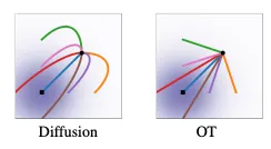
Note that the sections that follow are going to feel like a lot of math, but they are a windy path to get to a nice and easy-to-understand comparison with diffusion models, which is: If you write the steps that diffusion models take as an ODE, the line they trace to get to the final point is not straight; why not just make it straight? Neural networks probably like predicting straight lines. See Figure 3 from the flow matching paper below:

What is a continuous normalizing flow?

Continuous normalizing flows were first introduced in the paper Neural Ordinary Differential Equations. Consider the update rule of a recurrent neural network:

$\textbf{h}_{t + 1} = \textbf{h}_t + f(\textbf{h}_t, \theta_t)$

In a vanilla RNN, $f$ just does a matrix multiplication on $\textbf{h}_t$. This can be thought of as a discrete update rule over time. Neural ODEs are the continuous version of this:

$\frac{d \textbf{h}(t)}{dt} = f(\textbf{h}(t), t, \theta)$

The diffusion process described earlier can be conceptualized as a neural ODE - you just have to have an infinite number of infinitesimally small diffusion steps.

This formulation permits us to use any off-the-shelf ODE solver to generate samples from the distribution. The simplest method is to just sample some small $\Delta t$ and use Euler’s method to solve the ODE (as in the figure below).

How do we train a continuous normalizing flow?

Sampling from an ODE is fine. The real question is how we parameterize these, and what update rule we use to update the parameters.

The goal of the optimization is to make the output of our ODE solver close to our data. This can be formulated as:

$\mathcal{L}(z(t_1)) = \mathcal{L}\big( z(t_0) + \int_{t_0}^{t_1} f(z(t), t, \theta) \big)$

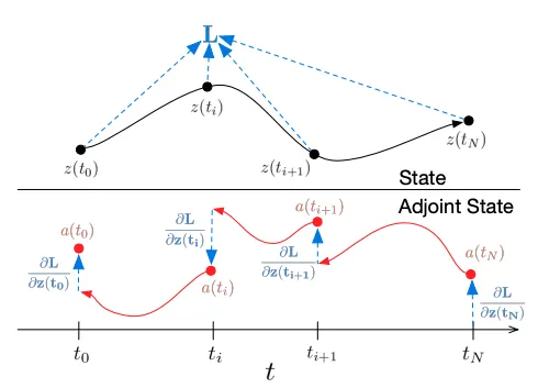
To optimize this, we need to know how $\mathcal{L}(z(t))$ changes with respect to $z(t)$:

$\begin{aligned} a(t) & = \frac{\partial \mathcal{L}(z(t))}{\partial z(t)} \\ \frac{d a(t)}{dt} & = -a(t)^T \frac{\partial f(z(t), t, \theta)}{\partial z} \\ \end{aligned}$

We can use the second equation to move backwards along $t$ using another ODE solver, back-propagating the loss at each step.

This function is called the adjoint, and is illustrated in Figure 2 from the original Neural ODE paper, copied below. It’s useful to know about but mainly as a barrier to overcome further down - we don’t want to actually use it because it is computationally expensive to unroll every time we want to update our model.

However, the above process can be computationally expensive to do; the analogy in our diffusion model would be having to update every single point along our diffusion trajectory on every update, each time using an ODE solver. Instead, the paper Flow Matching for Generative Modeling proposes a different approach, called Continuous Flow Matching (CFM).

What is continuous flow matching?

First, some terminology: the paper makes use of optimal transport to speed up the training process. This basically just means the most efficient way to move between two points given some constraints. Alternatively, it is the path which minimizes a total cost.

The goal of CFM is to avoid going through the entire ODE solver on every update step. Instead, in order to scale our flow matching model training, we want to be able to sample a single point, and then use optimal transport to move that point to the data distribution.

First, we can express our continuous normalizing flow as a function:

$\phi_t(x) : [0, 1] \times \mathbb{R}^d \rightarrow \mathbb{R}^d$

This can be read as, “a function mapping from a point in $\mathbb{R}^d$ (i.e., a $d$-dimensional vector) and a time between 0 and 1 to another point in $\mathbb{R}^d$”. We are interested in the first derivative of the function:

$\begin{aligned} v_t(\phi_t(x)) & = \frac{d}{dt} \phi_t(x) \\ \phi_0(x) & = x \\ \end{aligned}$

where $x = (x_1, \dots, x_d) \in \mathbb{R}^d$ are the points in the data distribution (for example, our images).

In a CNF, the function $v_t$, usually called the vector field, is parameterized by the neural network. Our goal is to update the neural network so that we can use it to move from some initial point sampled from a prior distribution to one of the points in our data distribution by using an ODE solver (in other words, by following the vector field).

Some more notation:

• $p_0$ is the prior distribution, usually a standard normal $\mathcal{N}(0, I)$
• $q$ is the true data distribution, which is unknown, but we get samples from it in the form of images (for example)
• $p_1$ is the posterior distribution, which we want to be close to $q$
• $p_t$ is the distribution of points at time $t$ between $p_0$ and $p_1$. Think of these as noisy images from somewhere along some path from our prior to posterior distributions.

How do we learn the vector field?

The goal of the learning process, as with most learning processes, is to maximize the likelihood of the data distribution. We can express this using the flow matching objective:

$\mathcal{L}_{FM}(\theta) = \mathbb{E}_{t,p_t(x)} || v_t(x) - u_t(x) ||^2$

where:

• $v_t$ is the output of the neural network for time $t$ and the data sample(s) $x$
• $u_t$ is the “true vector field” (i.e., the vector field that would take us from the prior distribution to the data distribution)

So the loss function is simply doing mean squared error between the neural network output and some “ground truth” vector field value. Seems simple enough, right? The problem is that we don’t really know what $p_t$ and $u_t$ are, since we could take many paths from $p_0$ to $p_1$.

The insight from this paper starts with the marginal probability path. This should be familiar if you are familiar with graphical models like conditional random fields. The idea is that, given some sample from our data distribution, we can marginalize $p_t$ over all the different ways we could get from $p_t$ to some sample in our data distribution:

$p_t(x) = \int p_t(x | x_1) q(x_1) dx_1$

This can be read as, “$p_t(x)$ is the distribution over all the noisy images that can be denoised to an image in our data distribution”.

We can also marginalize over the vector field:

$u_t(x) = \int u_t(x | x_1) \frac{p_t(x | x_1) q(x_1)}{p_t(x)} dx_1$

This can be read as, “$u_t(x)$ is the distribution over all the vector fields that could take us from a noisy image to an image in our data distribution, weighted by the probability of each path that the process would take”.

Rather than computing the (intractable) integrals in the equations above, we can instead condition on a single sample $x_1 \sim q(x_1)$, use that sample to get a noisy sample $x \sim p_t(x | x_1)$ and then use that noisy sample to compute the direction $u_t(x | x_1)$ that our vector field should take to recover the original image $x_1$, finally minimizing the conditional flow matching objective:

$\mathcal{L}_{CFM}(\theta) = \mathbb{E}_{t,q(x_1),p_t(x|x_1)} || v_t(x) - u_t(x | x_1) ||^2$

Without going into the math, the paper shows that this objective has the same gradients as the earlier objective, which is a pretty interesting result. It basically means that we can just follow our vector field from the original image to the noisy image, and that vector field is the optimal one to follow backwards to our original image.

The conditional path $p_t(x | x_1)$ is chosen to progressively add noise to the sample $x_1$ (this is what diffusion models do):

$p_t(x|x_1) = \mathcal{N}(x | \mu_t(x_1), \sigma_t(x_1)^2 I)$

where:

• $\mu_t$ is the time-dependent mean of the Gaussian distribution, ranging from $\mu_0(x_1) = 0$ (i.e., the prior is has mean 0) to $\mu_1(x_1) = x_1$ (i.e., the posterior is has mean $x_1$)
• $\theta_t$ is the time-dependent standard deviation, ranging from $\theta_0(x_1) = 1$ (i.e., the prior has standard deviation 1) to $\theta_1(x_1) = \sigma_{\text{min}}$ (i.e., the posterior has some very small amount of noise)

Using the above notation, the paper considers the flow:

$\phi_t(x) = \sigma_t(x_1)x + \mu_t(x_1)$

Remember that $\phi_t(x)$ is the flow at time $t$ for the sample $x$, meaning the point that we would get to if we followed the vector field from $x$ for time $t$ (in other words, the noisy image).

Recall from earlier that $u_t(\phi_t(x) | x_1)$ is just the derivative of this field, which gives us a closed form solution for our target values in our $\mathcal{L}_{CFM}$ objective:

$\begin{aligned} u_t(x|x_1) & = \frac{d}{dt} \phi_t(x) \\ & = \frac{\sigma_t'(x_1)}{\sigma_t(x_1)} (x - \mu_t(x_1)) + \mu_t'(x_1) \\ \end{aligned}$

where:

• $\sigma_t'(x_1)$ is the derivative of $\sigma_t(x_1)$ with respect to $t$
• $\mu_t'(x_1)$ is the derivative of $\mu_t(x_1)$ with respect to $t$

This is basically just a more general formulation of diffusion models. Specifically, diffusion models can be expressed as:

$\begin{aligned} \mu_t(x_1) & = \alpha_{1 - t}x_1 \\ \sigma_t(x_1) & = \sqrt{1 - \alpha_{1 - t}^2} \\ \end{aligned}$

although $\alpha$ here is slightly different from earlier.

Alternatively, the optimal transport conditioned vector field can be expressed as:

$\begin{aligned} \mu_t(x) & = t x_1 \\ \sigma_t(x) & = 1 - (1 - \sigma_{\text{min}}) t \\ \end{aligned}$

This vector field linearly scales the mean from the image down to 0, and linearly scales the standard deviation from $\sigma_{\text{min}}$ up to 1. This has the derivatives:

$\begin{aligned} \mu_t'(x) & = x_1 \\ \sigma_t'(x) & = -(1 - \sigma_{\text{min}}) \\ \end{aligned}$

Plugging into the above equation gives us $u_t(x | x_1)$ (don’t worry, it’s just basic algebra):

$\begin{aligned} u_t(x | x_1) & = \frac{-(1 - \sigma_{\text{min}})}{1 - (1 - \sigma_{\text{min}})t} (x - t x_1) + x_1 \\ & = \frac{-(1 - \sigma_{\text{min}}) x + t x_1 (1 - \sigma_{\text{min}}) + x_1 (1 - (1 - \sigma_{\text{min}}) t)}{1 - (1 - \sigma_{\text{min}}) t} \\ & = \frac{-(1 - \sigma_{\text{min}}) x + tx_1 - tx_1 \sigma_{\text{min}} + x_1 - tx_1 + tx_1 \sigma_{\text{min}}}{1 - (1 - \sigma_{\text{min}}) t} \\ & = \frac{x_1 - (1 - \sigma_{\text{min}}) x}{1 - (1 - \sigma_{\text{min}}) t} \end{aligned}$

So, to recap the learning procedure:

1. Choose a sample $x_1$ from the dataset.
2. Compute $u_t(x | x_1)$ using the equation above.
3. Predict $v_t(x | x_1)$ using the neural network.
4. Minimize the mean squared error between the two.

Then, sampling from the model is just a matter of following the flow from some random noise vector along the vector field predicted by the neural network, as you would with a regular ODE.

Specifically, they found that they were able to get good quality samples using a fixed-step ODE solver (the simplest kind) using $\leq 100$ steps.