Ben's Blog

Monotonic Attention

Write-up explaining an implementation of monotonic attention using a probabilistic graphical model.

Nov 09, 2023

If you want to try this out yourself, install the package here.

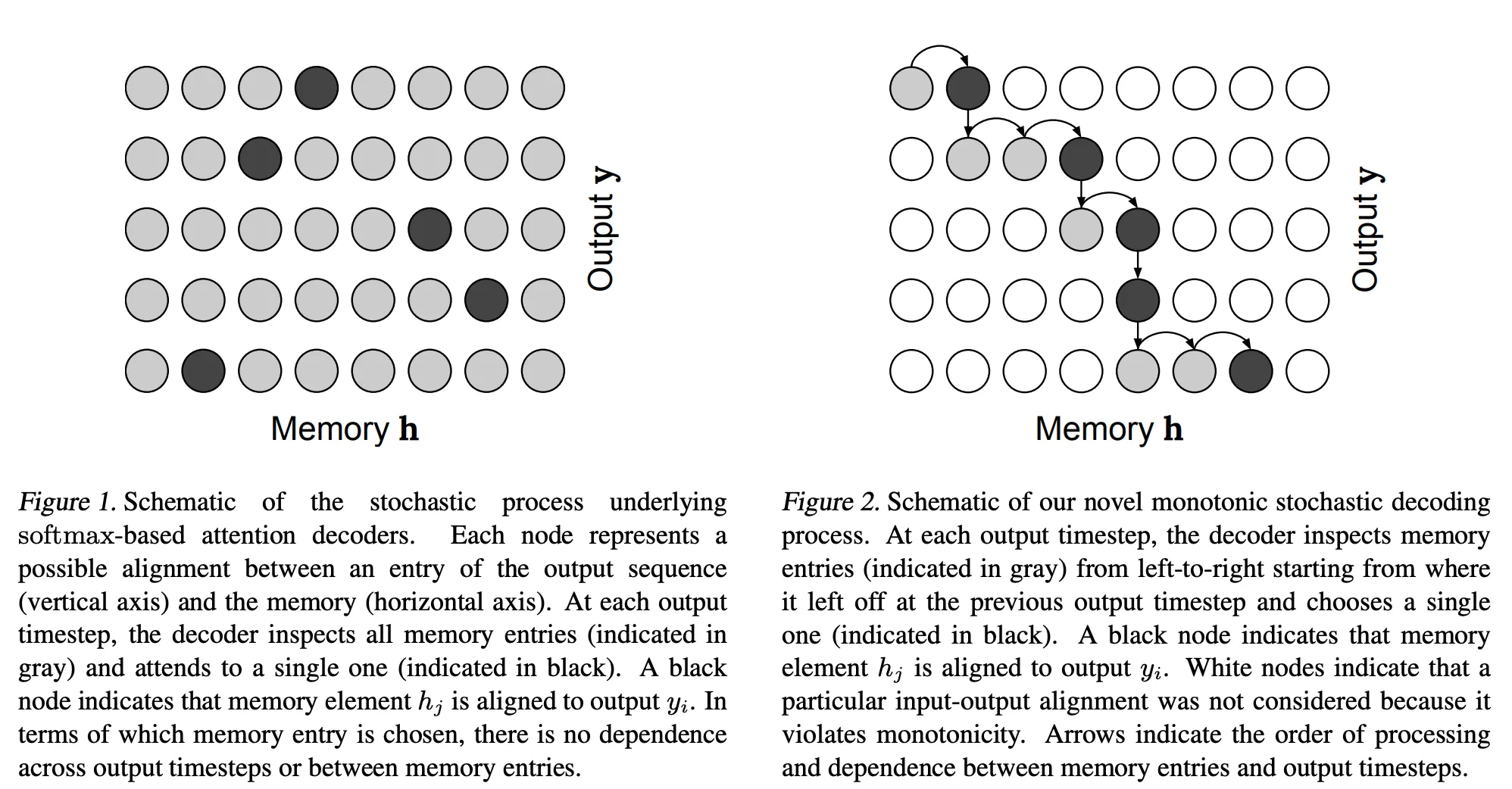
Monotonic attention describes a subclass of problems relating to constraining the attention weights of a neural network attention layer to have some beneficial properties. In the case of monotonic attention, this means constraining the mask to be monotonically increasing. This is well illustrated by Figures 1 and 2 from the paper Online and Linear-Time Attention by Enforcing Monotonic Alignments (2017).

Illustration of Monotonic Attention in Action

Why Monotonic Attention?

There are a number of modeling problems which are described well by monotonic relationships. For example:

ASR and TTS

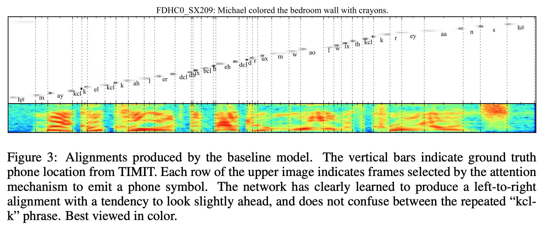
In automatic speech recognition (ASR) or text-to-speech (TTS), we want to align some audio waveform with some text representation. The words in the text are monotonically aligned with the audio waveform. Consider Figure 1 from Attention-Based Models for Speech Recognition (2015):

Figure 1 from Chorowski et. al. 2015

Machine Translation

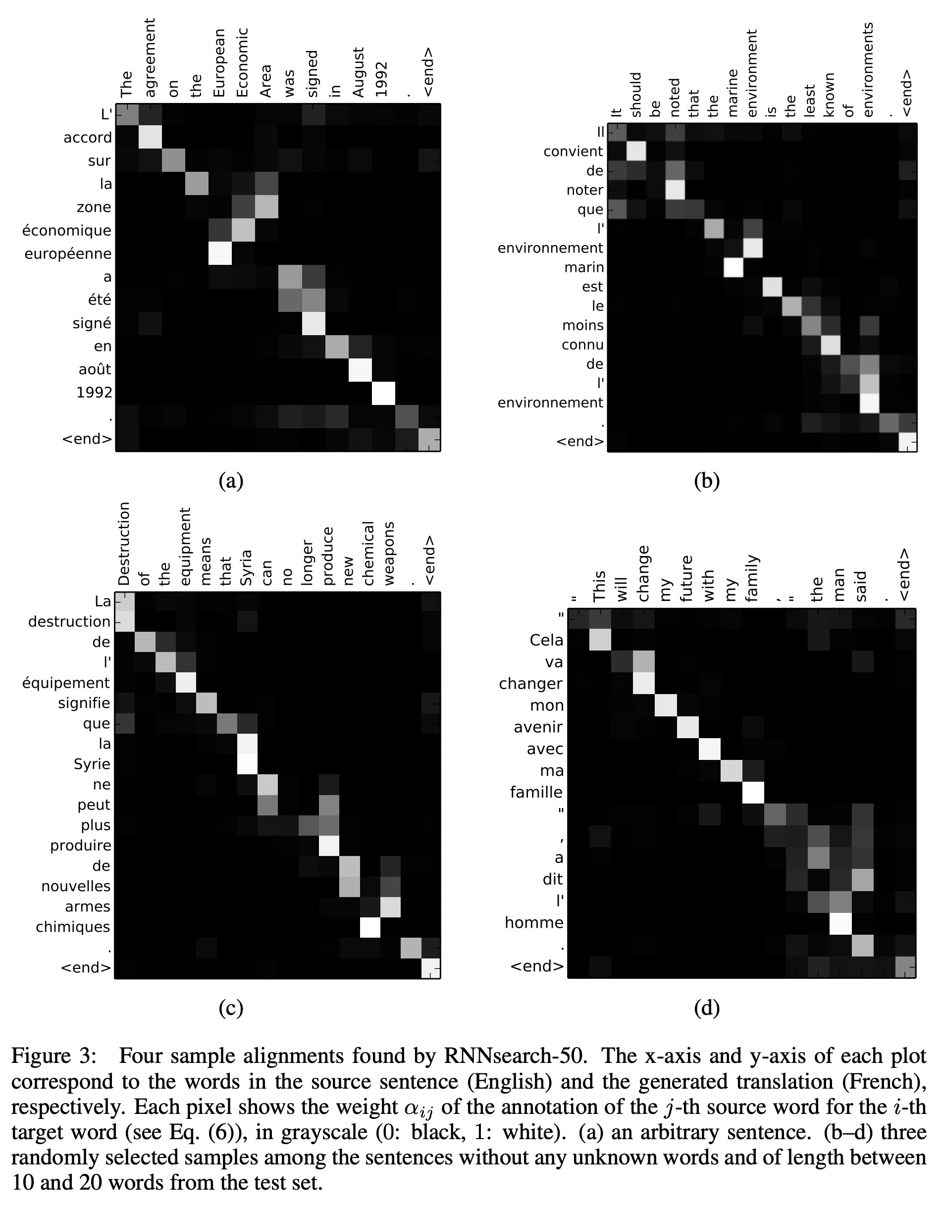
In machine translation, we want to align some source language with some target language. The words in the source language are often monotonically aligned with the words in the target language (although this is not always the case). Consider Figure 3 from Neural Machine Translation by Jointly Learning to Align and Translate (2016)

Figure 3 from Bahdanau et. al. (2016)

Summarization

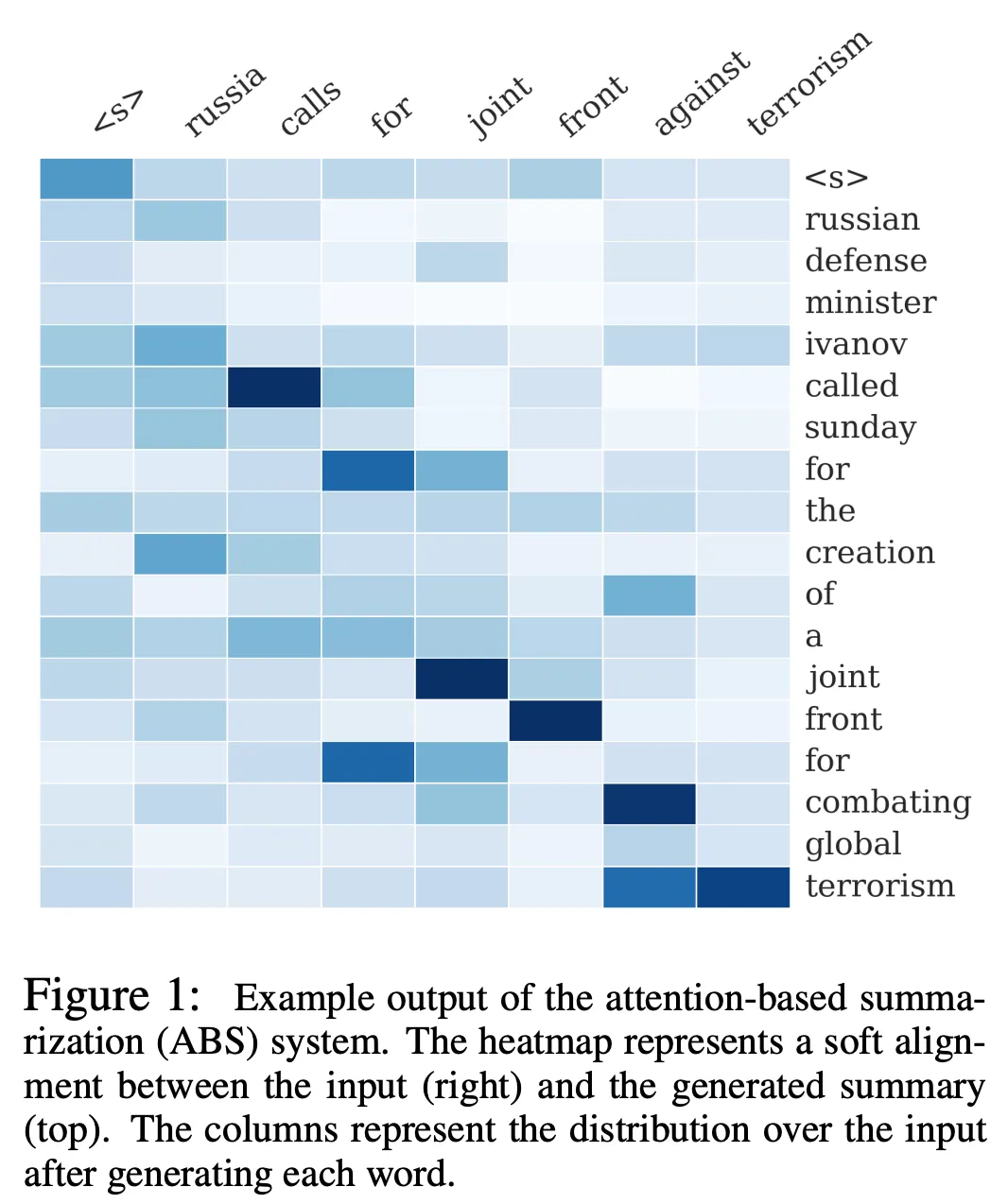
In summarization, the summary is often nearly monotonically-aligned with the source text. Consider Figure 1 from A Neural Attention Model for Abstractive Sentence Summarization (2015):

Figure 1 from Rush et. al. (2015)

Many-to-Many Monotonicity

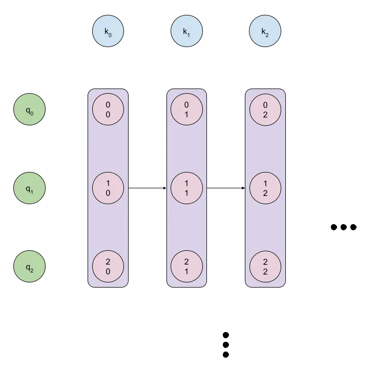
The first method for enforcing monotonicity that I’ll describe is a symmetric graphical model, where each node defines the probability of incrementing either the query or key index. To relate this approach to transformer-type self-attention, we’ll use the variables $q_i$ , $k_j$ and $v_j$ to represent the query, key and value vectors, with $T_i$ total query vectors and $T_j$ total key and value vectors, giving us the attention equation:

$\begin{aligned} \text{Attention}(Q, K, V) & = \text{softmax}(\frac{Q K^T}{\sqrt{d_k}}) V \\ a_i & = \sum_{j}^{T_j} \frac{e^{q_i k_j / \sqrt{d_k}}}{\sum_{j}^{T_j} e^{q_i k_j / \sqrt{d_k}}} v_j \end{aligned}$

The monotonic attention approach instead considers the $q_i k_j$ term as a probability distribution between advancing the query or key index. This can be written as

$p_{ij} = \sigma(q_i k_j)$

where $\sigma$ is the sigmoid function that constrains the values to between zero and one. So we’ll have $T_i T_j$ scalar probability values $p_{ij}$ , which we can consider as nodes in a directed graphical model. The picture below shows this model, with $p_{ij}$ being the probability of moving one step to the right, and the $1 - p_{ij}$ being the probability of moving one step down:

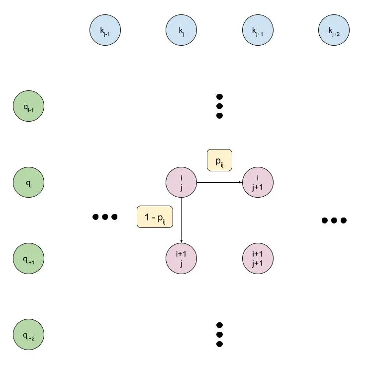
Monotonic attention graphical model

I’m calling this approach “Many-to-Many Monotonicity” because the model can relate an arbitrary number of keys to a single query, or an arbitrary number of queries to a single key, which provides less of an inductive bias than other approaches.

Training in Expectation

The above graphical model can be used to describe a probability distribution over all the monotonic paths from the top-left corner to the bottom-right corner. In order to train this model, we need to compute the marginal probability that a given node will be visited by a monotonic path.

To gain some intuition for what this means at training time:

We want to maximize the probability that good query-key pairs are visited by random paths through our graphical model, and minimize the probability that bad ones are visited.
The probability that a node is visited depends on the probability that it’s input nodes are visited, so we will need to backpropagate gradients to those inputs.

The next few sections of this post are going to get very math-heavy. People who have worked with graphical models before know how annoying it is to deal with the mathematics correctly, particularly when the math is not explained in sufficient detail, so I’m going to try to be as explicit as possible for anyone who wants to follow along. That being said, it’s probably not completely necessary to go through everything - the equations for the gradients, for example, can be verified numerically using finite differences, and the code can be verified using unit tests.

Forward Pass

To train this model, let’s start by writing the probability that node $(i, j)$ is included in a path as $\phi_{i, j}$ . We can then define the probability $\phi_{i + 1, j + 1}$ recurrently as:

$\phi_{i + 1, j + 1} = \phi_{i + 1, j} p_{i + 1, j} + \phi_{i, j + 1} (1 - p_{i, j + 1})$

We can write some simple PyTorch code to implement this:

def forward_pass_(probs: Tensor, phis: Tensor) -> None:
    for i in range(phis.size(-2)):
        for j in range(phis.size(-1)):
            if i == 0 and j == 0:
                phis[..., i, j] = 1.0
            elif i == 0:
                phis[..., i, j] = phis[..., i, j - 1] * probs[..., i, j - 1]
            elif j == 0:
                phis[..., i, j] = phis[..., i - 1, j] * (1 - probs[..., i - 1, j])
            else:
                phis[..., i, j] = (
                    phis[..., i, j - 1] * probs[..., i, j - 1] +
                    phis[..., i - 1, j] * (1 - probs[..., i - 1, j])
                )

Log-Space Forward Pass

Note that the above formulation has our probabilities being multiplied together many times, which lead to numerical underflow since we are using floating-point values. A small improvement is to therefore use log-probabilities rather than probabilities. This requires us to use the log-sum-exp function, which is defined as:

$\begin{aligned} \text{logsumexp}(a, b) & = \log(e^a + e^b) \\ & = \text{max}(a, b) + \log(e^{a - \text{max}(a, b)} + e^{b - \text{max}(a, b)}) \\ \end{aligned}$

We can then write:

$\log \phi_{i+1, j+1} = \text{logsumexp}(\log \phi_{i+1, j} + \log p_{i+1, j}, \log \phi_{i,j+1} + \log (1 - p_{i, j+1}))$

We can convert our above PyTorch implementation easily:

def _logaddexp(*ts: Tensor) -> Tensor:
    max_av = torch.stack(ts, dim=-1).max(dim=-1).values
    return max_av + torch.log(torch.stack([torch.exp(t - max_av) for t in ts], dim=-1).sum(dim=-1))

def _log_1mexp(x: Tensor) -> Tensor:
    return torch.log(-torch.expm1(x))  # log(1 - exp(x)), for computing log(1 - p)

def forward_pass_(probs: Tensor) -> Tensor:
    phis = torch.empty_like(probs)
    t_i, t_j = probs.size(-2), probs.size(-1)
    for i in range(t_i):
        for j in range(t_j):
            if i == 0 and j == 0:
                phis[..., i, j] = 1.0
            elif i == 0:
                phis[..., i, j] = phis[..., i, j - 1] * probs[..., i, j - 1]
            elif j == 0:
                phis[..., i, j] = phis[..., i - 1, j] * (1 - probs[..., i - 1, j])
            else:
                phis[..., i, j] = (
                    phis[..., i, j - 1] * probs[..., i, j - 1] +
                    phis[..., i - 1, j] * (1 - probs[..., i - 1, j])
                )
    return phis

Backward Pass

The gradients for this model are pretty straight-forward to compute. Recalling our forward pass equation:

$\phi_{i + 1, j + 1} = \phi_{i + 1, j} p_{i + 1, j} + \phi_{i, j + 1} (1 - p_{i, j + 1})$

We can write the gradients as:

$\begin{aligned} \frac{\partial \phi_{i + 1, j + 1}}{\partial p_{i + 1, j}} & = \phi_{i + 1, j} \\[1.5em] \frac{\partial \phi_{i + 1, j + 1}}{\partial \phi_{i + 1, j}} & = p_{i + 1, j} \\[1.5em] \frac{\partial \phi_{i + 1, j + 1}}{\partial p_{i, j + 1}} & = -\phi_{i, j + 1} \\[1.5em] \frac{\partial \phi_{i + 1, j + 1}}{\partial \phi_{i, j + 1}} & = 1 - p_{i, j + 1} \end{aligned}$

We can write some PyTorch code to implement this:

def backward_pass_(probs: Tensor, phis: Tensor, grad_phis: Tensor) -> Tensor:
    grad_probs = torch.empty_like(grad_phis)
    t_i, t_j = probs.size(-2), probs.size(-1)
    for i in range(t_i - 1, -1, - 1):
        for j in range(t_j - 1, -1, -1):
            if i == t_i - 1 and j == t_j - 1:
                grad_probs[..., i, j] = 0.0
            elif i == t_i - 1:
                grad_probs[..., i, j] = grad_phis[..., i, j + 1] * phis[..., i, j]
                grad_phis[..., i, j] += grad_phis[..., i, j + 1] * probs[..., i, j]
            elif j == t_j - 1:
                grad_probs[..., i, j] = grad_phis[..., i + 1, j] * -phis[..., i, j]
                grad_phis[..., i, j] += grad_phis[..., i + 1, j] * (1 - probs[..., i, j])
            else:
                grad_probs[..., i, j] = (
                    grad_phis[..., i, j + 1] * phis[..., i, j] +
                    grad_phis[..., i + 1, j] * -phis[..., i, j]
                )
                grad_phis[..., i, j] += (
                    grad_phis[..., i, j + 1] * probs[..., i, j] +
                    grad_phis[..., i + 1, j] * (1 - probs[..., i, j])
                )
    return grad_probs

Log-Space Backward Pass

The gradients for the log-space version slightly more complicated to compute. Recalling our log-space forward pass equation:

$\log \phi_{i+1, j+1} = \text{logsumexp}(\log \phi_{i+1, j} + \log p_{i+1, j}, \log \phi_{i,j+1} + \log (1 - p_{i+1, j}))$

Bearing in mind the gradient of the $\text{logsumexp}$ function:

$\frac{\partial \text{logsumexp(a, b)}}{\partial a} = \frac{e^a}{e^a + e^b} = \frac{1}{1 + e^{b - a}} = \sigma(a - b)$

If we define $y = \text{logsumexp}(a, b)$ , then we can rewrite the above equation as:

$\frac{\partial \text{y}}{\partial a} = \frac{e^a}{e^y} = e^{a - y}$

We can write:

$\begin{aligned} \frac{\partial \log \phi_{i+1,j+1}}{\partial \log p_{i+1, j}} & = \sigma(\log \phi_{i+1, j} + \log p_{i+1, j} - \log \phi_{i,j+1} - \log (1 - p_{i, j+1})) \\ & = e^{\log \phi_{i+1, j} + \log p_{i+1, j} - \log \phi_{i+1,j+1}} \\[1.5em] \frac{\partial \log \phi_{i+1,j+1}}{\partial \log \phi_{i+1, j}} & = \sigma(\log \phi_{i+1, j} + \log p_{i+1, j} - \log \phi_{i,j+1} - \log (1 - p_{i, j+1})) \\ & = e^{\log \phi_{i+1, j} + \log p_{i+1, j} - \log \phi_{i+1,j+1}} \\[1.5em] \frac{\partial \log \phi_{i+1,j+1}}{\partial \log (1 - p_{i, j+1})} & = \sigma(\log \phi_{i,j+1} + \log (1 - p_{i, j+1}) - \log \phi_{i+1, j} - \log p_{i+1, j}) \\ & = e^{\log \phi_{i,j+1} + \log (1 - p_{i, j+1}) - \log \phi_{i+1,j+1}} \\[1.5em] \frac{\partial \log \phi_{i+1,j+1}}{\partial \log \phi_{i, j+1}} & = \sigma(\log \phi_{i,j+1} + \log (1 - p_{i, j+1}) - \log \phi_{i+1, j} - \log p_{i+1, j}) \\ & = e^{\log \phi_{i,j+1} + \log (1 - p_{i, j+1}) - \log \phi_{i+1,j+1}} \\[1.5em] \frac{\partial \log (1 - p_{i,j+1})}{\partial \log p_{i,j+1}} & = \frac{1}{e^{\log p_{i, j+1}} - 1} + 1 \end{aligned}$

We can write some PyTorch code to implement this:

def _d_log_1emxp(x: Tensor) -> Tensor:
    return 1 + (1 / (torch.exp(x) - 1))

def backward_pass_(log_probs: Tensor, log_phis: Tensor, grad_log_phis: Tensor) -> Tensor:
    grad_log_probs = torch.empty_like(grad_log_phis)
    t_i, t_j = log_probs.size(-2), log_probs.size(-1)
    for i in range(t_i - 1, -1, -1):
        for j in range(t_j - 1, -1, -1):
            if i == t_i - 1 and j == t_j - 1:
                grad_log_probs[..., i, j] = 0.0
            elif i == t_i - 1:
                grad_log_probs[..., i, j] = grad_log_phis[..., i, j + 1] * torch.exp(log_phis[..., i, j] + log_probs[..., i, j] - log_phis[..., i, j + 1])
                grad_log_phis[..., i, j] += grad_log_phis[..., i, j + 1] * torch.exp(log_phis[..., i, j] + log_probs[..., i, j] - log_phis[..., i, j + 1])
            elif j == t_j - 1:
                grad_log_probs[..., i, j] = grad_log_phis[..., i + 1, j] * torch.exp(log_phis[..., i, j] + _log_1mexp(log_probs[..., i, j]) - log_phis[..., i + 1, j]) * _d_log_1emxp(log_probs[..., i, j])
                grad_log_phis[..., i, j] += grad_log_phis[..., i + 1, j] * torch.exp(log_phis[..., i, j] + _log_1mexp(log_probs[..., i, j]) - log_phis[..., i + 1, j])
            else:
                grad_log_probs[..., i, j] = (
                    grad_log_phis[..., i, j + 1] * torch.exp(log_phis[..., i, j] + log_probs[..., i, j] - log_phis[..., i, j + 1]) +
                    grad_log_phis[..., i + 1, j] * torch.exp(log_phis[..., i, j] + _log_1mexp(log_probs[..., i, j]) - log_phis[..., i + 1, j]) * _d_log_1emxp(log_probs[..., i, j])
                )
                grad_log_phis[..., i, j] += (
                    grad_log_phis[..., i, j + 1] * torch.exp(log_phis[..., i, j] + log_probs[..., i, j] - log_phis[..., i, j + 1]) +
                    grad_log_phis[..., i + 1, j] * torch.exp(log_phis[..., i, j] + _log_1mexp(log_probs[..., i, j]) - log_phis[..., i + 1, j])
                )
    return grad_log_probs

While we’ve solved the issue of numerical stability in the forward pass, we still have potential numerical stability issues in the backward pass. We can solve this using log-space gradient operations (I’ll just provide the code below without the associated equations):

def backward_pass_(log_probs: Tensor, log_phis: Tensor, grad_log_phis: Tensor) -> Tensor:
    grad_log_probs = torch.empty_like(grad_log_phis)
    t_i, t_j = log_probs.size(-2), log_probs.size(-1)
    log_grad_log_phis = grad_log_phis.log()
    for i in range(t_i - 1, -1, -1):
        for j in range(t_j - 1, -1, -1):
            if i == t_i - 1 and j == t_j - 1:
                grad_log_probs[..., i, j] = 0.0
            elif i == t_i - 1:
                grad_log_probs[..., i, j] = (
                    log_grad_log_phis[..., i, j + 1]
                    + log_phis[..., i, j]
                    + log_probs[..., i, j]
                    - log_phis[..., i, j + 1]
                ).exp()
                log_grad_log_phis[..., i, j] = _logaddexp(
                    [
                        log_grad_log_phis[..., i, j],
                        log_grad_log_phis[..., i, j + 1]
                        + log_phis[..., i, j]
                        + log_probs[..., i, j]
                        - log_phis[..., i, j + 1],
                    ]
                )
            elif j == t_j - 1:
                grad_log_probs[..., i, j] = (
                    log_grad_log_phis[..., i + 1, j]
                    + log_phis[..., i, j]
                    + _log_1mexp(log_probs[..., i, j])
                    - log_phis[..., i + 1, j]
                ).exp() * _d_log_1emxp(log_probs[..., i, j])
                log_grad_log_phis[..., i, j] = _logaddexp(
                    [
                        log_grad_log_phis[..., i, j],
                        log_grad_log_phis[..., i + 1, j]
                        + log_phis[..., i, j]
                        + _log_1mexp(log_probs[..., i, j])
                        - log_phis[..., i + 1, j],
                    ]
                )
            else:
                grad_log_probs[..., i, j] = (
                    log_grad_log_phis[..., i, j + 1]
                    + log_phis[..., i, j]
                    + log_probs[..., i, j]
                    - log_phis[..., i, j + 1]
                ).exp() + (
                    log_grad_log_phis[..., i + 1, j]
                    + log_phis[..., i, j]
                    + _log_1mexp(log_probs[..., i, j])
                    - log_phis[..., i + 1, j]
                ).exp() * _d_log_1emxp(
                    log_probs[..., i, j]
                )
                log_grad_log_phis[..., i, j] = _logaddexp(
                    [
                        log_grad_log_phis[..., i, j],
                        log_grad_log_phis[..., i, j + 1]
                        + log_phis[..., i, j]
                        + log_probs[..., i, j]
                        - log_phis[..., i, j + 1],
                        log_grad_log_phis[..., i + 1, j]
                        + log_phis[..., i, j]
                        + _log_1mexp(log_probs[..., i, j])
                        - log_phis[..., i + 1, j],
                    ]
                )
    return grad_log_probs

A caveat to the above approach is that, since we’re taking the log of the gradients, we will actually need to backpropagate the positive and negative gradients separately. This can introduce additional computational overhead.

Parallelism (Making Training Go Brr)

Okay, so we’ve got a numerically-stable PyTorch implementation. Unfortunately, as written, it is very anti-PyTorch. We’re basically serially visiting each node in the graph, meaning it will be snail-like if we try to run it on a GPU. However, we can see that there’s some parallelism in both the forward and backward passes.

Intuition

It’s probably easiest to visualize how our algorithm can be parallelized using the diagram below:

Monotonic attention parallelism

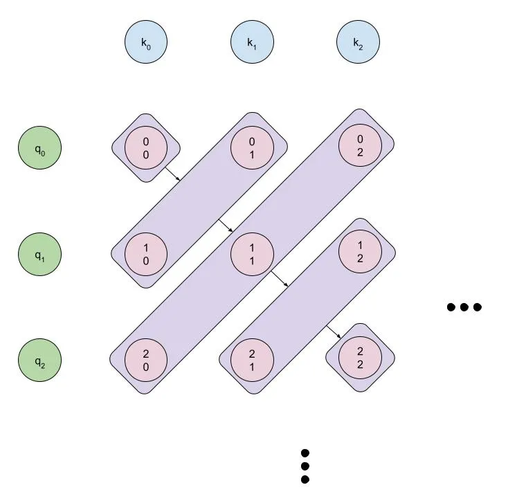
We can parallelize both the forward and backward passes over the diagonal of the matrix, but we’ll need to be careful about how we do it.

Forward Pass

Here’s a more parallel implementation of the forward pass:

def forward_pass_(log_probs: Tensor) -> Tensor:
    log_phis = torch.empty_like(log_probs)
    t_i, t_j = log_probs.size(-2), log_probs.size(-1)
    log_probs_padded = F.pad(log_probs, (1, 0, 1, 0), value=float("-inf"))
    log_probs_padded_1mexp = F.pad(_log_1mexp(log_probs), (1, 0, 1, 0), value=float("-inf"))
    log_phis[..., 0, 0] = 0.0
    log_phis = F.pad(log_phis, (1, 0, 1, 0), value=float("-inf"))
    for t in range(1, t_i + t_j - 1):
        i = torch.arange(max(0, t - t_j + 1), min(t + 1, t_i))
        j = torch.arange(min(t, t_j - 1), max(-1, t - t_i), -1)
        log_phis[..., i + 1, j + 1] = _logaddexp(
            log_phis[..., i + 1, j] + log_probs_padded[..., i + 1, j],
            log_phis[..., i, j + 1] + log_probs_padded_1mexp[..., i, j + 1],
        )
    return log_phis[..., 1:, 1:]

It’s nice when the parallel implementation is cleaner than the serial one, although I find it easier to follow the logic for the serial one (maybe it’s from doing too many programming competitions).

Note that in the implementation above, instead of special-casing the edge points, we add a padding dimension to the probability matrix representing 0 probability (which, in log-space, is negative infinity).

Backward Pass

The parallel implementation of the backwards pass is similar.

def backward_pass_(log_probs: Tensor, log_phis: Tensor, grad_log_phis: Tensor) -> Tensor:
    grad_log_probs = torch.empty_like(grad_log_phis)
    t_i, t_j = log_probs.size(-2), log_probs.size(-1)
    grad_log_phis = F.pad(grad_log_phis, (0, 1, 0, 1), value=0.0)
    log_phis = F.pad(log_phis, (0, 1, 0, 1), value=0.0)
    grad_log_probs[..., t_i - 1, t_j - 1] = 0.0

    for t in range(t_i + t_j - 2, -1, -1):
        i = torch.arange(max(0, t - t_j + 1), min(t + 1, t_i))
        j = torch.arange(min(t, t_j - 1), max(-1, t - t_i), -1)

        grad_log_probs[..., i, j] = grad_log_phis[..., i, j + 1] * (
            log_phis[..., i, j] + log_probs[..., i, j] - log_phis[..., i, j + 1]
        ).exp() + grad_log_phis[..., i + 1, j] * (
            log_phis[..., i, j] + _log_1mexp(log_probs[..., i, j]) - log_phis[..., i + 1, j]
        ).exp() * _d_log_1emxp(
            log_probs[..., i, j]
        )

        grad_log_phis[..., i, j] += (
            grad_log_phis[..., i, j + 1] * (log_phis[..., i, j] + log_probs[..., i, j] - log_phis[..., i, j + 1]).exp()
            + grad_log_phis[..., i + 1, j]
            * (log_phis[..., i, j] + _log_1mexp(log_probs[..., i, j]) - log_phis[..., i + 1, j]).exp()
        )

    return grad_log_probs

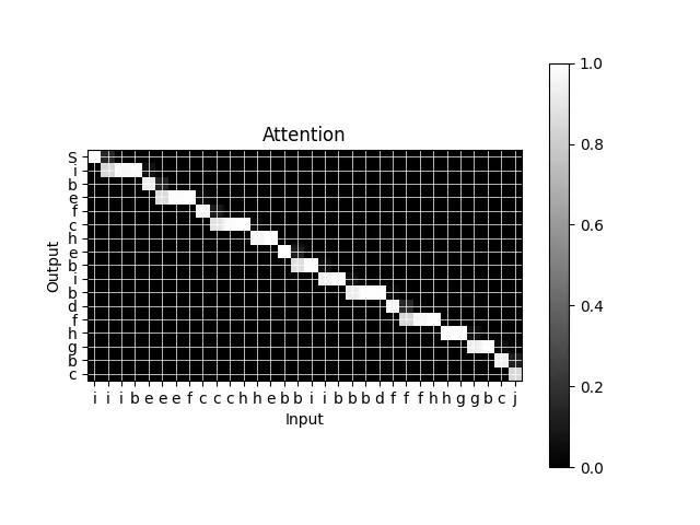
Toy Example

I trained a toy model to verify that my implementation is working as intended. The model takes a sequence of letters as input, and outputs a sequence of letters by first de-duplicating adjacent letters, then repeating the unique letter some number of times. This is a good task for a monotonic attention model to learn.

# mypy: disable-error-code="import-not-found"
"""Defines a dummy "letters" model.

This model takes a random sequence of letters and outputs a new sequence
containing the unique letters repeated N times. For example, the input sequence
"abbbccdef" would be transformed into "aabbccddeeff".
"""

import argparse
import itertools
import random
from typing import Iterator

import numpy as np
import torch
import torch.nn.functional as F
from torch import Tensor, nn, optim
from torch.utils.data.dataloader import DataLoader
from torch.utils.data.dataset import IterableDataset

from monotonic_attention import MultiheadMonotonicAttention

try:
    import matplotlib.pyplot as plt
except ModuleNotFoundError:
    raise ModuleNotFoundError("Visualization requires matplotlib: `pip install matplotlib`")


class LettersDataset(IterableDataset[tuple[Tensor, Tensor]]):
    def __init__(self, num_letters: int, seq_length: int, num_reps: int) -> None:
        super().__init__()

        assert 2 <= num_letters <= 26, f"`{num_letters=}` must be between 2 and 26"

        self.num_letters = num_letters
        self.seq_length = seq_length
        self.num_reps = num_reps
        self.padding_idx = 0

        self.vocab = list("abcdefghijklmnopqrstuvwxyz"[:num_letters])

    def tokenize(self, s: str) -> Tensor:
        return Tensor([self.vocab.index(c) + 1 for c in s])

    def detokenize(self, t: Tensor) -> str:
        return "".join(self.vocab[int(i) - 1] for i in t.tolist())

    @property
    def vocab_size(self) -> int:
        return self.num_letters + 1

    def __iter__(self) -> Iterator[tuple[Tensor, Tensor]]:
        return self

    def __next__(self) -> tuple[Tensor, Tensor]:
        tokens_in: list[int] = []
        tokens_out: list[int] = []
        prev_letter: int | None = None
        while len(tokens_in) < self.seq_length:
            choices = [i for i in range(1, self.num_letters + 1) if i != prev_letter]
            letter = random.choice(choices)
            prev_letter = letter
            tokens_in.extend([letter] * random.randint(1, min(self.seq_length - len(tokens_in), self.num_reps * 2)))
            tokens_out.extend([letter] * self.num_reps)

        tokens_in_t = torch.tensor(tokens_in)
        tokens_out_t = torch.tensor(tokens_out)
        return tokens_in_t, tokens_out_t

    def collate_fn(self, items: list[tuple[Tensor, Tensor]]) -> tuple[Tensor, Tensor]:
        tokens_in, tokens_out = zip(*items)

        # Pads the output tokens and creates a mask.
        max_out_len = max(len(t) for t in tokens_out)
        tokens_out_t = torch.full((len(tokens_out), max_out_len), fill_value=self.padding_idx, dtype=torch.long)
        for i, token_out in enumerate(tokens_out):
            tokens_out_t[i, : len(token_out)] = token_out

        return torch.stack(tokens_in), tokens_out_t


class MonotonicSeq2Seq(nn.Module):
    """Defines a monotonic sequence-to-sequence model.

    Parameters:
        vocab_size: The vocabulary size
        dim: The number of embedding dimensions
    """

    def __init__(self, vocab_size: int, dim: int, padding_idx: int, use_rnn: bool) -> None:
        super().__init__()

        self.vocab_size = vocab_size
        self.embs = nn.Embedding(vocab_size, dim, padding_idx=padding_idx)
        self.init_emb = nn.Parameter(torch.zeros(1, 1, dim))
        self.rnn = nn.LSTM(dim, dim, batch_first=True) if use_rnn else None
        self.attn = MultiheadMonotonicAttention(dim, num_heads=1)
        self.proj = nn.Linear(dim, vocab_size)

    def forward(self, src: Tensor, tgt: Tensor) -> Tensor:
        bsz = tgt.size(0)
        src_emb = self.embs(src)
        tgt_emb = torch.cat((self.init_emb.expand(bsz, -1, -1), self.embs(tgt[..., :-1])), dim=1)
        x = self.attn(tgt_emb, src_emb, src_emb)
        if self.rnn is not None:
            x, _ = self.rnn(x)
        x = self.proj(x)
        return x

    def get_attention_matrix(self, src: Tensor, tgt: Tensor) -> Tensor:
        bsz = tgt.size(0)
        src_emb = self.embs(src)
        tgt_emb = torch.cat((self.init_emb.expand(bsz, -1, -1), self.embs(tgt[..., :-1])), dim=1)
        return self.attn.get_attn_matrix(tgt_emb, src_emb)


def train(
    num_letters: int,
    seq_length: int,
    num_reps: int,
    batch_size: int,
    device_type: str,
    embedding_dims: int,
    max_steps: int,
    save_path: str | None,
    use_rnn: bool,
) -> None:
    device = torch.device(device_type)

    ds = LettersDataset(num_letters, seq_length, num_reps)
    dl = DataLoader(ds, batch_size=batch_size, collate_fn=ds.collate_fn)
    pad = ds.padding_idx

    model = MonotonicSeq2Seq(ds.vocab_size, embedding_dims, pad, use_rnn)
    model.to(device)

    opt = optim.Adam(model.parameters(), lr=1e-3)

    for i, (tokens_in, tokens_out) in itertools.islice(enumerate(dl), max_steps):
        opt.zero_grad(set_to_none=True)
        tokens_in, tokens_out = tokens_in.to(device), tokens_out.to(device)
        tokens_out_pred = model(tokens_in, tokens_out)
        loss = F.cross_entropy(tokens_out_pred.view(-1, ds.vocab_size), tokens_out.view(-1), ignore_index=pad)
        loss.backward()
        opt.step()
        print(f"{i}: {loss.item()}")

    # Gets the attention matrix.
    tokens_in, tokens_out = next(ds)
    tokens_in = tokens_in.unsqueeze(0).to(device)
    tokens_out = tokens_out.unsqueeze(0).to(device)
    attn_matrix = model.get_attention_matrix(tokens_in, tokens_out)
    attn_matrix = attn_matrix[0, 0, 0].detach().cpu().numpy()

    # Visualize the attention matrix against the letters.
    letters_in = ds.detokenize(tokens_in[0])
    letters_out = "S" + ds.detokenize(tokens_out[0])[:-1]
    plt.figure()
    plt.imshow(attn_matrix, cmap="gray")
    plt.xticks(range(len(letters_in)), letters_in)
    plt.yticks(range(len(letters_out)), letters_out)
    plt.xlabel("Input")
    plt.ylabel("Output")
    plt.title("Attention")
    plt.colorbar()

    # Grid between adjacent cells.
    for i in range(len(letters_in)):
        plt.axvline(i, color="white", linewidth=0.5)
    for i in range(len(letters_out)):
        plt.axhline(i, color="white", linewidth=0.5)

    if save_path is not None:
        plt.savefig(save_path, bbox_inches="tight")
    else:
        plt.show()


def main() -> None:
    random.seed(1337)
    torch.manual_seed(1337)
    np.random.seed(1337)

    parser = argparse.ArgumentParser(description="Train a dummy letters model.")
    parser.add_argument("-n", "--num-letters", type=int, default=10, help="How many unique letters to use")
    parser.add_argument("-r", "--num-reps", type=int, default=3, help="How many repetitions in the output sequence")
    parser.add_argument("-b", "--batch-size", type=int, default=16, help="The batch size to use")
    parser.add_argument("-s", "--seq-length", type=int, default=32, help="Input sequence length")
    parser.add_argument("-d", "--device", type=str, default="cpu", help="The device to use for training")
    parser.add_argument("-e", "--embedding-dims", type=int, default=32, help="Number of embedding dimensions")
    parser.add_argument("-m", "--max-steps", type=int, default=100, help="Maximum number of steps to train for")
    parser.add_argument("-p", "--save-path", type=str, default=None, help="Where to save the visualized attentions")
    parser.add_argument("-u", "--use-rnn", action="store_true", help="Whether to use an RNN")
    args = parser.parse_args()

    train(
        num_letters=args.num_letters,
        num_reps=args.num_reps,
        batch_size=args.batch_size,
        seq_length=args.seq_length,
        device_type=args.device,
        embedding_dims=args.embedding_dims,
        max_steps=args.max_steps,
        save_path=args.save_path,
        use_rnn=args.use_rnn,
    )


if __name__ == "__main__":
    # python -m examples.letters
    main()

When I visualize the attention mask for the model, sure enough, it looks like it’s learning the correct correspondence between letters:

Toy problem

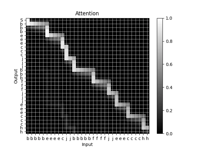
Note that this visualization is showing the marginal probabilities for each cell, which is why the path is not a pure solid line.

Making It Faster

The next step, if we were to try and use this mechanism in a real model, would be to make it faster by writing a custom CUDA kernel for the forward and backward passes. However, with the parallelism we described earlier, we run into a slight annoyance, because the number of parallel operations is not constant; we have one operation on the first step, two operations on the second step, and so on. This will lead to pretty poor GPU utilization. This fact will motivate the modification I’ll describe the next section.

One-To-Many Monotonicity

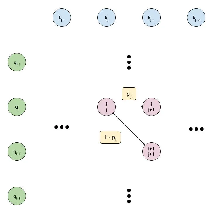
Motivated by the difficulty of writing a high-performance CUDA kernel for the many-to-many monotonic attention mechanism, we can make a slight modification to the graphical model which will ultimately let us write an efficient kernel. As with earlier, it’s easiest to understand this modification by looking at a diagram:

One-to-many monotonic attention graphical model

Some points of note:

The choice of key or query as the direction which is constantly being incremented is now dependent on the type of model we want to build. For example, in the diagram above, we constantly increment the key, meaning that each key can correspond to at most one query. This could be used in a speech-to-text model, for example, where each step of the output (the audio waveform or spectrogram, for instance) basically depends on exactly one step of the input (the text token).
Related to above, the graphical model is now no longer symmetric, since we are enforcing that either the key or query is constantly incremented. However, the choice is arbitrary and can be swapped if necessary.
Each node depends only on the nodes to the left of it, so we can scan from left-to-right rather than from the top left corner to the bottom right corner. This means that:
1. The number of parallel steps being performed remains constant, rather than changing size.
2. We’ll have only $T_i$ or $T_j$ parallel steps rather than $T_i + T_j - 1$ . This is a minor point since for practical applications we expect either $T_i >> T_j$ or vice versa, but it is a minor optimization.

Parallelism

Rather than messing around with the foundational math as we did with the earlier operations, I’ll just skip to implementing the optimal version of the code, since the math is basically quite similar. Note that we now have the parallel groups visualized in the diagram below:

One-to-many monotonic attention parallelism

This will be easier to ultimately convert to a CUDA kernel.

Forward Pass

The PyTorch code to implement the forward pass for our one-to-many monotonic attention model is relatively simpler than with our many-to-many model:

def forward_pass_(log_probs: Tensor) -> Tensor:
    log_phis = torch.empty_like(log_probs)
    t_i = log_probs.size(-2)
    log_phis[..., 0, :] = float("-inf")
    log_phis[..., 0, 0] = 0.0
    for i in range(1, t_i):
        log_phis[..., i, 0] = log_phis[..., i - 1, 0] + log_probs[..., i - 1, 0]
        log_phis[..., i, 1:] = _logaddexp(
            log_phis[..., i - 1, 1:] + log_probs[..., i - 1, 1:],
            log_phis[..., i - 1, :-1] + _log_1mexp(log_probs[..., i - 1, :-1]),
        )
    return log_phis

Some notes about this implementation:

We increment over the second-to-last dimension to keep memory accesses contiguous.
Rather than using a padding dimension, as in the earlier implementation, we just do a separate operation for the operations which have a diagonal predecessor.

Backward Pass

Similarly, our backward pass is also simpler:

def backward_pass_(log_probs: Tensor, log_phis: Tensor, grad_log_phis: Tensor) -> Tensor:
    grad_log_probs = torch.empty_like(grad_log_phis)
    t_i = log_probs.size(-2)
    grad_log_probs[..., t_i - 1, :] = 0.0
    for i in range(t_i - 2, -1, -1):
        p = log_phis[..., i + 1, :].clamp_min(MIN_LOG_PROB)
        a = (log_phis[..., i, :] + log_probs[..., i, :] - p).exp()
        b = (log_phis[..., i, :-1] + _log_1mexp(log_probs[..., i, :-1]) - p[..., 1:]).exp()
        c = grad_log_phis[..., i + 1, :] * a
        d = grad_log_phis[..., i + 1, 1:] * b
        grad_log_probs[..., i, :] = c
        grad_log_probs[..., i, :-1] += d * _d_log_1emxp(log_probs[..., i, :-1])
        grad_log_phis[..., i, :] += c
        grad_log_phis[..., i, :-1] += d
    return grad_log_probs

Checking for Correctness

As a point of note regarding verifying that these implementations are all correct, here’s how we can write a unit test to verify the backward pass. First, define a custom PyTorch function:

class MonotonicAttention(Function):
    @staticmethod
    def forward(ctx: FunctionCtx, log_probs: Tensor) -> Tensor:
        log_phis = forward_pass_(log_probs)
        ctx.save_for_backward(log_probs, log_phis)
        return log_phis

    @staticmethod
    @once_differentiable
    def backward(ctx: FunctionCtx, grad_log_phis: Tensor) -> Tensor:
        log_probs, log_phis = ctx.saved_tensors
        grad_log_probs = backward_pass_(log_probs, log_phis, grad_log_phis.clone())
        return grad_log_probs

def monotonic_attention(probs: Tensor, epsilon: float = 1e-3) -> Tensor:
    """Computes the monotonic attention normalization on the transition probabilities.

    Args:
        probs: The transition probabilities, with shape
            ``(bsz, tsz_src, tsz_tgt)`` and values in ``[0, 1]``.
        epsilon: The epsilon value to use for the normalization.

    Returns:
        The marginalized probabilities for each cell being part of a monotonic
        alignment path, with shape ``(bsz, tsz_src, tsz_tgt)`` and values in
        ``[0, 1]``.
    """
    tsz_src, tsz_tgt = probs.size(-2), probs.size(-1)
    if tsz_tgt > tsz_src:
        warnings.warn("One-to-many attention expects the source sequence to be longer than the target sequence!")
    probs = (probs * (1 - 2 * epsilon)) + epsilon
    return MonotonicAttention.apply(probs.log()).exp()

Next, we can use torch.autograd.gradcheck to verify that our analytic backwards pass matches the backwards pass computed using finite difference approximation:

def test_cpu_simple() -> None:
    bsz, tsz_src, tsz_tgt = 2, 7, 5
    probs = torch.rand(bsz, tsz_src, tsz_tgt, dtype=torch.double)

    # Tests the forward pass.
    phis = monotonic_attention_log(probs)
    assert (phis >= 0).all()
    assert (phis <= 1).all()

    # Tests the backward pass using finite differences.
    probs.requires_grad_(True)
    torch.autograd.gradcheck(monotonic_attention_log, probs, fast_mode=True)

Toy Problem

We’ll verify this implementation on another toy problem. This is similar to the first toy problem, except that we restrict the output to have only one unique letter at a time.

Toy problem 2

Sure enough, after training the marginal probabilities form a many-to-one mapping from the inputs to the outputs.

CUDA Kernel (Making Training Go BRRRRRRR)

As mentioned earlier, the reason for using the one-to-many version of the monotonic attention mechanism instead of the many-to-many version is because we can write a more performant CUDA kernel. Actually, I’m going to use Triton, because I used it for another project recently and found the developer experience to be way nicer than writing a CUDA kernel in C++. I’ll provide the code for the forward and backward passes together, with some comments on how it works.

Forward Pass

@triton.jit
def logaddexp(a, b):
    max_ab = tl.maximum(a, b)
    return max_ab + tl.math.log(tl.math.exp(a - max_ab) + tl.math.exp(b - max_ab))


@triton.jit
def log_1mexp(x):
    return tl.log(-tl.math.expm1(x))


@triton.jit
def d_log_1mexp(x):
    return 1 + (1 / tl.math.expm1(x))


@triton.jit
def forward_pass_kernel(
    # Log probabilities tensor (input)
    log_probs_ptr,
    log_probs_s_bsz,
    log_probs_s_src,
    log_probs_s_tgt,
    # Log phis tensor (output)
    log_phis_ptr,
    log_phis_s_bsz,
    log_phis_s_src,
    log_phis_s_tgt,
    # Tensor dimensions
    t_i,
    t_j,
    BLOCK_SIZE_C: tl.constexpr,
):
    # Parallelize over the batch dimension.
    b_idx = tl.program_id(0)
    j_idx = tl.program_id(1)

    # Pointers to the log probabilities.
    j = (j_idx * BLOCK_SIZE_C) + tl.arange(0, BLOCK_SIZE_C)
    jmask = j < t_j
    jmask_shifted = jmask & (j > 0)

    # Gets pointers offset for the current batch.
    log_probs_ptr = log_probs_ptr + b_idx * log_probs_s_bsz
    log_phis_ptr = log_phis_ptr + b_idx * log_phis_s_bsz

    # Accumulator for the log phis.
    log_phis_acc = tl.where(j == 0, 0.0, tl.full((BLOCK_SIZE_C,), value=NEG_INF, dtype=tl.float32))

    # Stores first log phi value.
    log_phis_first_ptr = log_phis_ptr + j * log_phis_s_tgt
    tl.store(log_phis_first_ptr, log_phis_acc, mask=jmask)
    tl.debug_barrier()

    for i in range(1, t_i):
        log_probs_prev_ptr = log_probs_ptr + (i - 1) * log_probs_s_src + j * log_probs_s_tgt
        log_probs_prev = tl.load(log_probs_prev_ptr, mask=jmask)

        log_phis_prev_m1_ptr = log_phis_ptr + (i - 1) * log_phis_s_src + (j - 1) * log_phis_s_tgt
        log_probs_prev_m1_ptr = log_probs_ptr + (i - 1) * log_probs_s_src + (j - 1) * log_probs_s_tgt
        log_phis_prev_m1 = tl.load(log_phis_prev_m1_ptr, mask=jmask_shifted, other=NEG_INF)
        log_probs_prev_m1 = tl.load(log_probs_prev_m1_ptr, mask=jmask_shifted, other=NEG_INF)

        log_phis_a = log_phis_prev_m1 + log_1mexp(log_probs_prev_m1)
        log_phis_b = log_phis_acc + log_probs_prev
        log_phis_acc = logaddexp(log_phis_a, log_phis_b).to(tl.float32)

        log_phis_next_ptr = log_phis_ptr + i * log_phis_s_src + j * log_phis_s_tgt
        tl.store(log_phis_next_ptr, log_phis_acc, mask=jmask)

        # Barrier to ensure that we can access the stored log phis from the
        # adjacent thread in the next iteration.
        tl.debug_barrier()

Backward Pass

@triton.jit
def backward_pass_kernel(
    # Log probabilities tensor (input)
    log_probs_ptr,
    log_probs_stride_bsz,
    log_probs_stride_src,
    log_probs_stride_tgt,
    # Log phis tensor (input)
    log_phis_ptr,
    log_phis_s_bsz,
    log_phis_s_src,
    log_phis_s_tgt,
    # Gradient of log phis tensor (input)
    grad_log_phis_ptr,
    grad_log_phis_s_bsz,
    grad_log_phis_s_src,
    grad_log_phis_s_tgt,
    # Gradient of log probabilities tensor (output)
    grad_log_probs_ptr,
    grad_log_probs_s_bsz,
    grad_log_probs_s_src,
    grad_log_probs_s_tgt,
    # Tensor dimensions
    t_i,
    t_j,
    BLOCK_SIZE_C: tl.constexpr,
):
    # Parallelize over the batch dimension.
    b_idx = tl.program_id(0)
    j_idx = tl.program_id(1)

    # Pointers to the log probabilities.
    j = (j_idx * BLOCK_SIZE_C) + tl.arange(0, BLOCK_SIZE_C)
    jmask = j < t_j
    jmask_shifted = j < (t_j - 1)

    # Gets pointers offset for the current batch.
    log_probs_ptr = log_probs_ptr + b_idx * log_probs_stride_bsz
    log_phis_ptr = log_phis_ptr + b_idx * log_phis_s_bsz
    grad_log_phis_ptr = grad_log_phis_ptr + b_idx * grad_log_phis_s_bsz
    grad_log_probs_ptr = grad_log_probs_ptr + b_idx * grad_log_probs_s_bsz

    # Stores first log phi value.
    grad_log_probs_last_ptr = grad_log_probs_ptr + (t_i - 1) * log_phis_s_src + j * log_phis_s_tgt
    tl.store(grad_log_probs_last_ptr, tl.zeros((BLOCK_SIZE_C,), dtype=tl.float32), mask=j < t_j)
    tl.debug_barrier()

    for i in range(t_i - 2, -1, -1):
        # log_phis[..., i + 1, :]
        log_phis_next_ptr = log_phis_ptr + (i + 1) * log_phis_s_src + j * log_phis_s_tgt
        log_phis_next = tl.load(log_phis_next_ptr, mask=jmask)

        # log_phis[..., i + 1, 1:]
        log_phis_next_p1_ptr = log_phis_ptr + (i + 1) * log_phis_s_src + (j + 1) * log_phis_s_tgt
        log_phis_next_p1 = tl.load(log_phis_next_p1_ptr, mask=jmask_shifted)

        # log_phis[..., i, :]
        log_phis_cur_ptr = log_phis_ptr + i * log_phis_s_src + j * log_phis_s_tgt
        log_phis_cur = tl.load(log_phis_cur_ptr, mask=jmask)

        # log_probs[..., i, :]
        log_probs_cur_ptr = log_probs_ptr + i * log_probs_stride_src + j * log_probs_stride_tgt
        log_probs_cur = tl.load(log_probs_cur_ptr, mask=jmask)

        # grad_log_phis[..., i + 1, :]
        grad_log_phis_next_ptr = grad_log_phis_ptr + (i + 1) * grad_log_phis_s_src + j * grad_log_phis_s_tgt
        grad_log_phis_next = tl.load(grad_log_phis_next_ptr, mask=jmask)

        # grad_log_phis[..., i + 1, 1:]
        grad_log_phis_next_p1_ptr = grad_log_phis_ptr + (i + 1) * grad_log_phis_s_src + (j + 1) * grad_log_phis_s_tgt
        grad_log_phis_next_p1 = tl.load(grad_log_phis_next_p1_ptr, mask=jmask_shifted)

        # grad_log_probs[..., i, :]
        grad_log_probs_cur_ptr = grad_log_probs_ptr + i * grad_log_probs_s_src + j * grad_log_probs_s_tgt

        # grad_log_phis[..., i, :]
        grad_log_phis_cur_ptr = grad_log_phis_ptr + i * grad_log_phis_s_src + j * grad_log_phis_s_tgt
        grad_log_phis_cur = tl.load(grad_log_phis_cur_ptr, mask=jmask)

        # Computes the new values.
        a = tl.math.exp(log_phis_cur + log_probs_cur - log_phis_next)
        b = tl.math.exp(log_phis_cur + log_1mexp(log_probs_cur) - log_phis_next_p1)
        c = grad_log_phis_next * a
        d = grad_log_phis_next_p1 * b
        grad_log_probs_cur = tl.where(jmask_shifted, c + d * d_log_1mexp(log_probs_cur), c)
        grad_log_phis_cur = grad_log_phis_cur + tl.where(jmask_shifted, c + d, c)

        # Stores the new values.
        tl.store(grad_log_probs_cur_ptr, grad_log_probs_cur, mask=jmask)
        tl.store(grad_log_phis_cur_ptr, grad_log_phis_cur, mask=jmask)

        # Barrier to ensure that we can access the stored log phis from the
        # adjacent thread in the next iteration.
        tl.debug_barrier()

Comments

The above code should be relatively easy to follow if you compare it with the original PyTorch implementations. Triton abstracts a lot of stuff that’s happening under-the-hood. The most tricky thing about converting the PyTorch functions to Triton kernels is handling handling the “previous diagonal value” problem. Thinking in CUDA terms, each of our $T_j$ values are being processed in separate threads, each of which we will denote $j$ , over $T_i$ timesteps, each of which we will denote $i$ . A given value for node $(i, j)$ depends on the values for $(i - 1, j)$ and $(i - 1, j - 1)$ . We don’t have to worry about the value $(i - 1, j)$ since that value was computed in the same thread, but we do have to worry about the value $(i - 1, j - 1)$ because it was computed in a different thread, meaning we will have to communicate between threads.

In my mental model of Triton, it should handle this inter-thread communication for us. If we were doing this in CUDA, we keep our values in shared memory, and use __syncthreads() after writing to shared memory to ensure that we don’t have any synchronization issues. This depends on our block size being larger than $T_j$ , but this is a reasonable expectation because we expect $T_i >> T_j$ for most problems we deal with. The CUDA kernels above will probably have some unexpected behavior for longer sequence lengths.